Image 1: Okavango Delta May 25th, 2019
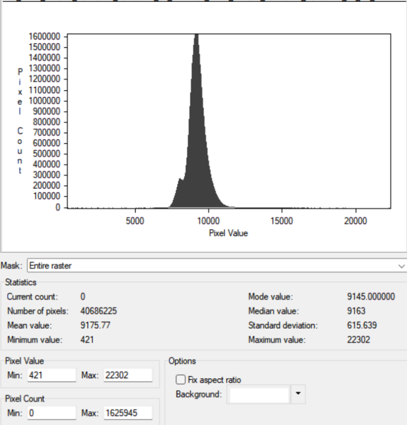
To describe the Landsat 8 Coastal Aerosol band (Band 1), we look at the image statistics and the histogram distribution provided in the data. This band is made up of 40,806,347 pixels with a mean value of 8,654.38 and a median of 8,713. The histogram shows a very sharp, narrow peak centred around the mode value of 8,783.00, indicating that the vast majority of the pixel values are tightly clustered in a small range. Although the values range from a minimum of 202 to a maximum of 41,190, the concentration of data in such a tiny area tells us that the raw image has extremely low contrast. To improve the visual quality of this band, a linear contrast stretch is a necessary enhancement. This process takes the narrow range of values where most of the data is located and spreads them out across the full range of the display. The reason for this is that the Coastal Aerosol band is designed to pick up subtle differences in shallow water or atmospheric particles, but these details are hidden when the brightness levels are so similar. By stretching the contrast, it can make these small differences visible, allowing us to distinguish between different features that would otherwise look like a single shade of dark gray.
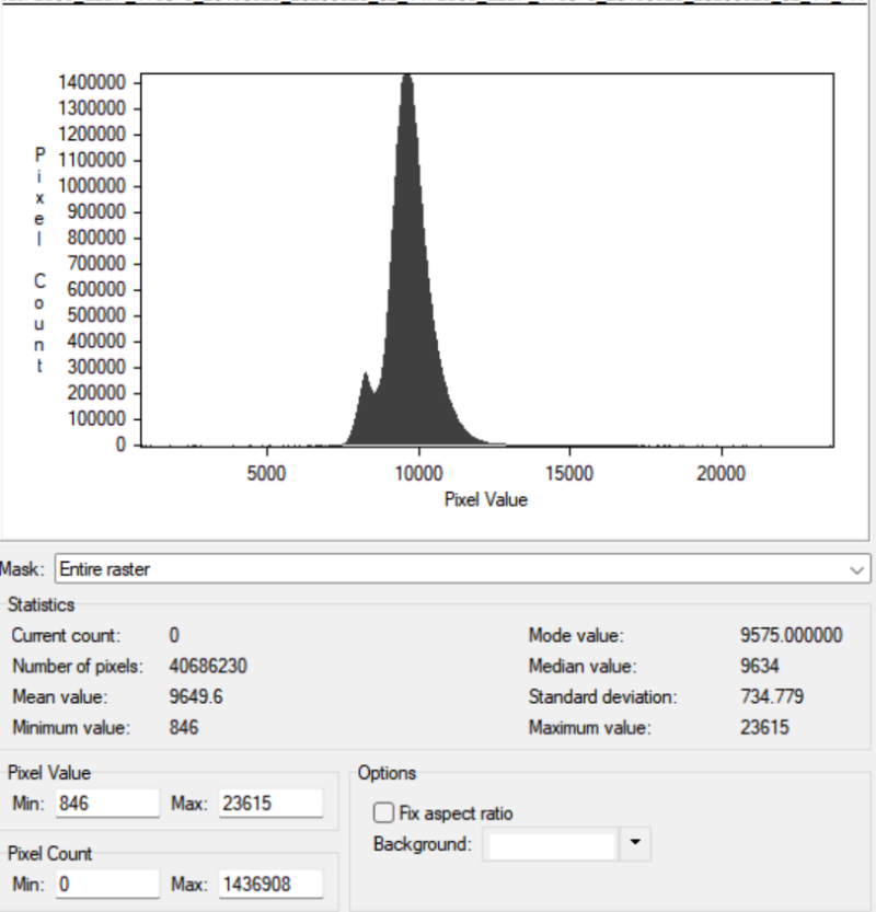
Looking at the blue band (Band 2) for this Landsat 8 scene, the statistics reveal a dataset that is heavily clustered within a narrow range. The mean value of 9,649.6 and a median of 9,634 are very close, which tells us that the data is relatively balanced around its center. However, the standard deviation of 734.78 is quite small compared to the full range of possible values, which extends from a minimum of 846 to a maximum of 23,615. This indicates that while there are a few very bright pixels—likely representing highly reflective surfaces or small clouds—the vast majority of the landscape is reflecting blue light at a very similar intensity. In a raw state, this makes the image appear flat because the useful information is squeezed into a tiny portion of the available spectrum. The histogram provides a clear visual map of this distribution, showing a sharp, tall peak between the 8,000 and 11,000 range. You can also spot a smaller shoulder or secondary bump on the left side of the main peak, which accounts for the darker features in the image, such as the water in the river channel or the dense vegetation along the banks. Because so much of the data is concentrated in one spot, the image lacks the necessary contrast to distinguish fine details between different types of soil or vegetation. The long tail stretching toward the maximum value of 23,615 shows that there is a lot of empty space in the higher brightness levels that isn't being used effectively for the majority of the terrain. To improve the visual quality of this band, a contrast enhancement—specifically a linear stretch—is essential. By "stretching" the narrow peak of the histogram so that it fills the entire display range, we can force the subtle differences in pixel values to become more visible to the human eye. This process would involve remapping the lower values (around 8,000) to black and the moderately high values (around 12,000) to white. Doing this would broaden the visual range, making the river stand out sharply against the land and revealing textures in the dry surrounding areas that are currently hidden in a muddy grey. Without these adjustments, the image remains difficult to interpret because the human eye cannot easily perceive the tiny numerical differences between the pixels in that central cluster.
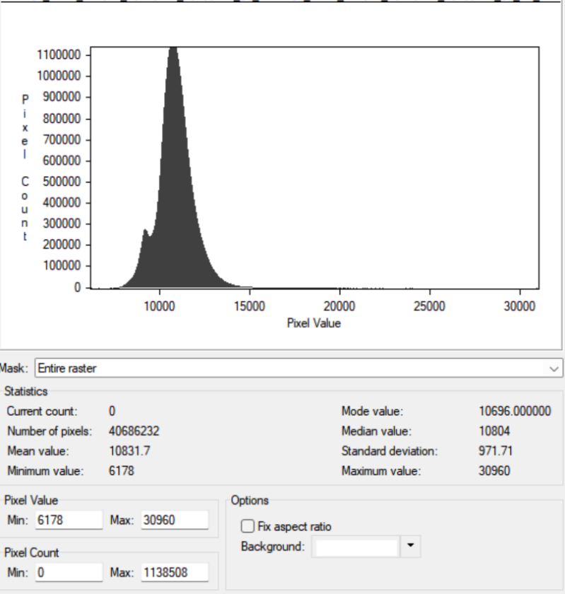
The statistics for the green band (Band 3) of this Landsat 8 image show a dataset that is concentrated within a specific, narrow range of brightness values. With a mean of 10,831.7 and a median of 10,804, the data points are closely grouped together, suggesting that most of the landscape reflects green light at a very similar level. While the total range spans from a minimum of 6,178 to a maximum of 30,960, the standard deviation is only 971.71. This low deviation tells us that the image naturally lacks high contrast, as the vast majority of the over 40 million pixels are not utilizing the full available dynamic range. The histogram provides a visual map of this behaviour, featuring a single, tall peak that dominates the center of the graph. On the lower end of the scale, there is a small shoulder or secondary bump, which likely represents the darker, less reflective portions of the scene, such as the water or deep shadows within the river delta. Conversely, the long, thin tail extending toward the maximum value of 30,960 indicates the presence of a few highly reflective features, perhaps bare sand or small clouds. Because the bulk of the data is squeezed into such a small section of the histogram, the raw image appears flat and muddy, making it difficult to distinguish between different types of vegetation or soil moisture levels. To improve the visual quality of the green band, a contrast enhancement—specifically a linear or standard deviation stretch—is highly recommended. By stretching the narrow cluster of values to fill the entire display range (from 0 to 255 for standard screens), we can amplify the subtle differences between pixels. This process is necessary because it allows the human eye to perceive fine details and textures in the landscape that are currently hidden in the narrow peak of the histogram. Enhancing the image in this way transforms the data from a dull, gray-toned capture into a crisp visual product where the river's path and the surrounding terrain become clearly defined.

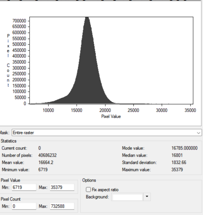
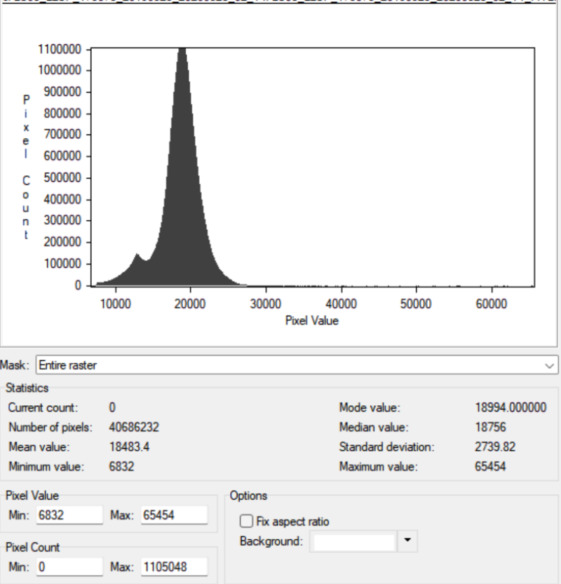
The Short-Wave Infrared 1 (SWIR 1) band (Band 6) for this Landsat 8 image shows a much wider variety of data than the visible color bands. The average brightness value is 18,483.4, with a middle value of 18,756, which is significantly higher than the green or red bands. What makes this band stand out is its large standard deviation of 2,739.82, indicating that the differences between the darkest and brightest features are very sharp. While the total range is huge—stretching from a low of 6,832 to a maximum of 65,454—most of the landscape is still concentrated within a specific portion of that scale. The histogram for the SWIR 1 band features a tall, sharp peak that represents the most common ground types in the scene. To the left of this main peak, there is a very clear secondary "bump," which represents the features that absorb short-wave light, such as the moisture in the river and the wet soil in the delta. On the right side, a very long, thin tail reaches toward the highest values, likely representing extremely dry or reflective surfaces like bare rock or sand. Because the data is spread across a larger range than the visible bands, we can already see more detail here, but the image still feels "dark" because the brightest pixels (up to 65,454) are very rare, making the rest of the image look dim by comparison. To make this data useful for the human eye, a histogram equalization or a standard deviation stretch is the best choice. This enhancement would redistribute the clumped-up pixels across the entire display range, which is necessary because SWIR light is excellent for seeing through haze and identifying differences in soil and rock that look the same in regular color. By stretching the data, the wet areas of the river will look much darker and the dry land will look much brighter, creating a high-contrast map that clearly defines the geography of the area.
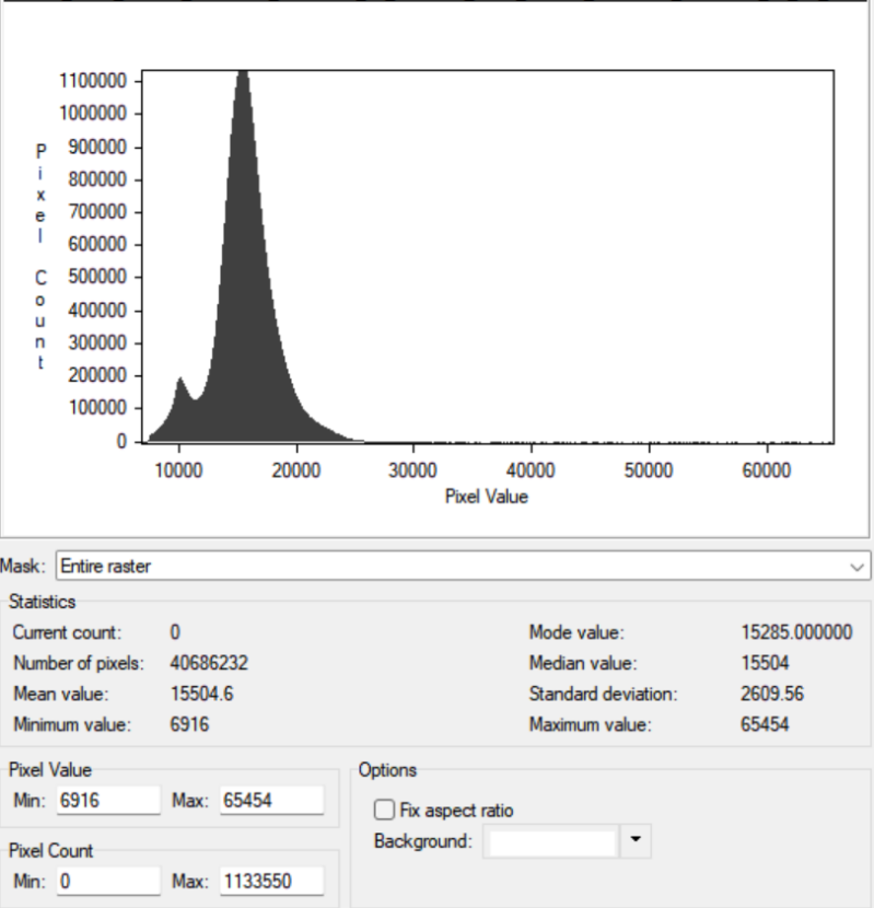
The Short-Wave Infrared 2 (SWIR 2) band (Band 7) of this Landsat 8 image shows data that is uniquely sensitive to different types of ground cover and moisture levels. The statistics show an average brightness of 15,504.6 and a median value of 15,504. With a standard deviation of 2,609.56, this band has a wide variety of values, second only to the SWIR 1 band in how spread out the data is. While the total range spans from a minimum of 6,916 to a maximum of 65,454, the vast majority of the over 40 million pixels are clustered in a much smaller area. This tells us that while most of the land reflects a similar amount of light, there are specific spots—like very dry rocks or wet soil—that stand out clearly. The histogram for this band features a tall, sharp peak with a very clear smaller "bump" on the left side. This smaller bump is important because it represents features that absorb a lot of short-wave light, particularly the water in the river and areas with high soil moisture. On the right side of the main peak, there is a very long, faint tail reaching toward the highest values, which likely shows bright, dry surfaces or bare earth. Because the main peak is quite narrow, the raw image looks very dark and lacks crisp details. It is hard to see the difference between various types of dry land because those pixels are all squeezed into the same middle range of the graph. To fix this and make the image look much better, a standard deviation stretch is the best enhancement to use. This process takes the main group of pixels and stretches them across the full range of dark to light. This is necessary because the SWIR 2 band is great for seeing through dust or haze and finding differences in rock types or soil wetness. By stretching the data, the wet areas of the river will look much darker, and the dry, rocky areas will look much brighter, creating a clear and sharp map that is much easier for a person to understand.
Image 2: Okavango Delta May 19th, 2025

To describe the Landsat 9 Coastal Aerosol band (Band 1), we first look at the basic image statistics and the distribution shown in the histogram. The dataset contains over 40 million pixels with a mean value of 8654.38 and a median of 8713. The histogram shows a very narrow, tall peak concentrated between the values of 7500 and 10000, which indicates that most of the image has very similar brightness levels. While the total range of possible values for this 16-bit data is quite large, the actual data is "bunched up" in a small area, which is why the original image appears dark and lacks clear detail. The presence of a small secondary peak on the left side of the main spike suggests there are some distinct features, likely darker areas like water or deep shadows, but they are not easily visible in the current state. Because the data is so tightly clustered, the visual quality of the image is poor. To fix this, a contrast enhancement or linear stretch is necessary. By stretching the narrow range of values (roughly 7000 to 11000) to fill the entire display range, we can bring out the hidden details in the landscape. This is a common step in remote sensing because it makes it much easier for the human eye to distinguish between different types of ground cover. Without these enhancements, the subtle differences in the Coastal Aerosol band remain hidden, making the data difficult to interpret for any real-world mapping or analysis.

To describe the Landsat 9 Blue band (Band 2), we look at the image statistics and the histogram distribution provided. This band contains 40,806,348 pixels with a mean value of 8965.65 and a median of 9000. Much like the previous band, the histogram shows a very sharp and narrow peak, with the majority of pixel values concentrated between 7500 and 11000. While the data ranges from a minimum of 1013 to a maximum of 46218, the vast majority of the information is crowded into a tiny fraction of the available 16-bit space. This tells us that the raw image lacks contrast, appearing very dark and flat to the human eye because the brightness levels are too similar. To improve the visual quality, a linear contrast stretch is necessary. Because the data is so tightly "bunched" around the mode value of 9048, we need to stretch this narrow range to cover the full display spectrum (0–255 for most screens). This enhancement is vital because it expands the subtle differences in brightness, allowing features like soil patterns or water edges to become visible. Without this step, the image remains a dark, uninterpretable block of pixels, as the human eye cannot distinguish between such small variations in digital values.
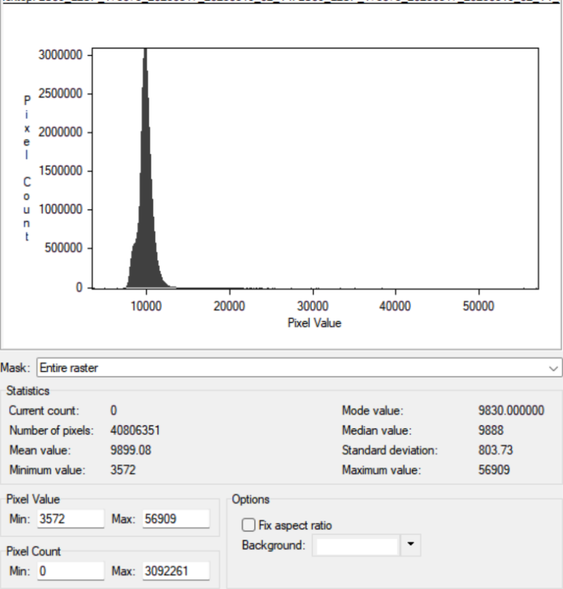
To describe the Landsat 9 Green band (Band 3), we examine the provided image statistics and the histogram distribution. This band consists of 40,806,351 pixels with a mean value of 9899.08 and a median of 9888. Looking at the histogram, we see a very sharp, narrow spike, indicating that the vast majority of pixel values are clustered tightly between 8000 and 12000. Although the data has a minimum value of 3572 and a maximum of 56909, the concentration around the mode of 9830 suggests that the raw image has very low contrast. Without processing, the image likely appears dark and lacks clear definition because the brightness levels of different ground features are too similar to be easily distinguished by the human eye. To improve the visual quality of this band, a contrast enhancement, such as a linear stretch, is necessary. By taking the narrow range where most data resides and stretching it to fill the full display spectrum, we can make subtle details—like vegetation health or sediment in water—much more apparent. This reasoning is based on the fact that while the sensor captures a high range of values, the actual scene content occupies only a small portion of that range. Enhancing the image in this way is essential for any meaningful visual interpretation or mapping task.
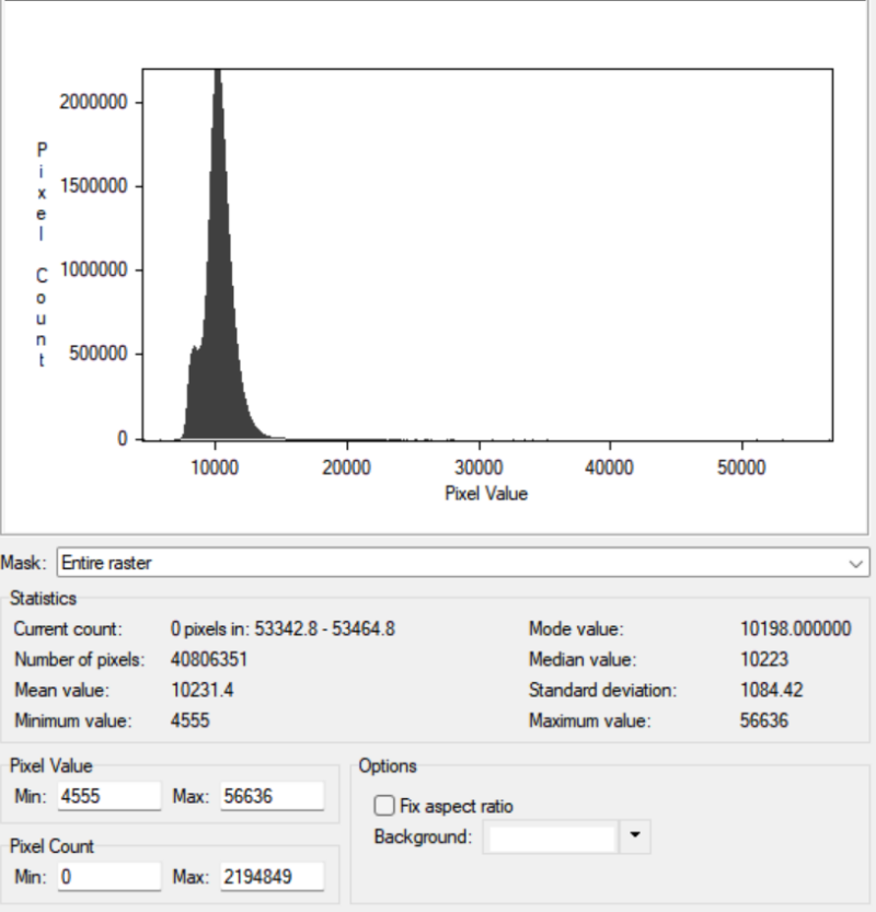
To describe the Landsat 9 Red band (Band 4), we look at the image statistics and the histogram shape provided in the data. This band is made up of 40,806,351 pixels with a mean value of 10231.4 and a median of 10223. The histogram shows a very tall, narrow peak, which tells us that almost all the information in the image is gathered in a small range of brightness levels around the mode of 10198. While the values technically go as high as 56636, the vast majority of the data is squeezed between roughly 8000 and 15000. This clustering means the raw image has very little contrast and likely looks very dark or muddy, as the differences between ground features are too small to see clearly. To improve the visual quality of the Red band, a linear contrast stretch should be used. This enhancement takes the narrow group of values where the "action" is and spreads them out across the full range of the display. We need to do this because the human eye cannot distinguish between the subtle shades shown in the current, narrow histogram. By stretching the data, we can reveal the distinct shapes of land features and separate different types of soil or vegetation that currently look exactly the same. This process is necessary to turn the raw digital numbers into a clear, usable picture.
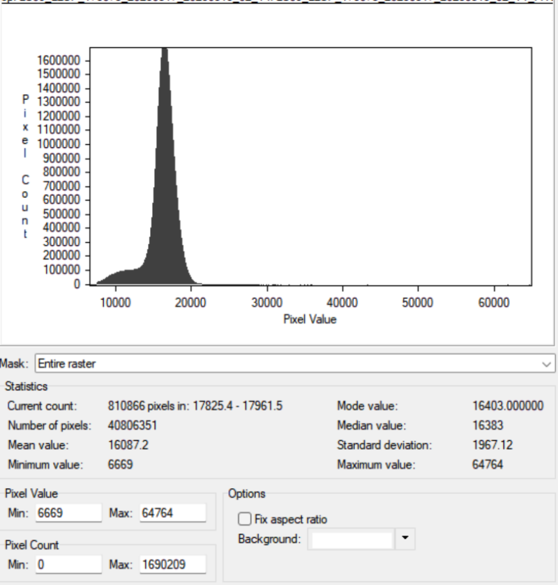
To describe the Landsat 9 Near-Infrared band (Band 5), we analyze the image statistics and the histogram provided in the data. This band is made up of 40,806,351 pixels with a mean value of 16087.2 and a median of 16383. Looking at the histogram, we see a very distinct, narrow peak centered around the mode value of 16403. While the values in this band are much higher than those in the visible light bands—which is normal since vegetation reflects Near-Infrared very strongly—the data is still very "bunched up" within a small range. With a minimum of 6669 and a maximum of 64764, most of the actual image information occupies only a tiny slice of the possible brightness levels, leading to an image that lacks clear detail and contrast. To improve the visual quality, a linear contrast stretch is highly recommended. This process takes the narrow cluster of values seen in the histogram and spreads them across the full range of the display. This enhancement is vital for the Near-Infrared band because it helps us see the subtle differences in plant health and water boundaries that are currently hidden. Without stretching the data, the image looks flat and greyish, making it very difficult for anyone to tell the difference between a thick forest and a grassy field. By expanding the contrast, these important land features become sharp and easy to identify.
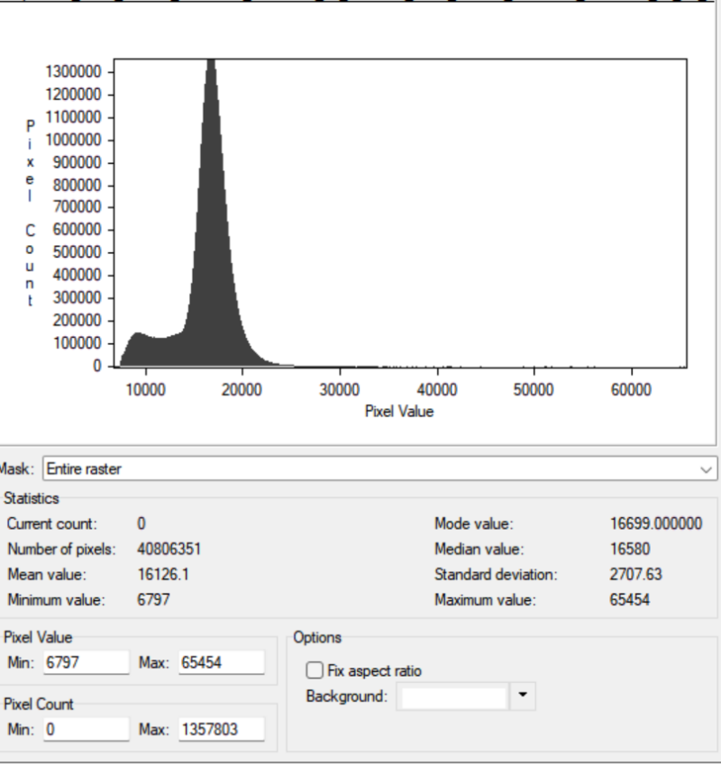
To describe the Landsat 9 Shortwave Infrared 1 band (Band 6), we look at the image statistics and the histogram provided in the data. This band is composed of 40,806,351 pixels with a mean value of 16126.1 and a median of 16580. The histogram shows a primary peak at a mode of 16699, but it also features a smaller "shoulder" or secondary cluster of lower values around 10,000. Although the data technically spans from a minimum of 6797 to a maximum of 65454, the vast majority of the information is concentrated within a relatively narrow range. This tells us that the raw image lacks significant contrast; because the pixel values are so close together, the image would appear very dark and flat, making it difficult to distinguish between different types of terrain or soil moisture levels. To improve the visual quality of this band, a linear contrast stretch is a necessary enhancement. This process takes the specific range where most of the pixel values are clustered and expands them to fill the entire brightness scale of a display monitor. My reasoning for this is that SWIR 1 is particularly sensitive to moisture and geological features, but these details are currently "hidden" because the brightness levels are too similar for the human eye to separate. By stretching the contrast, we can clearly see the differences between wet and dry areas or different rock types that would otherwise look like a single, solid shade of dark gray. This step is essential for turning raw sensor data into an image that can be easily interpreted for land use or environmental study.
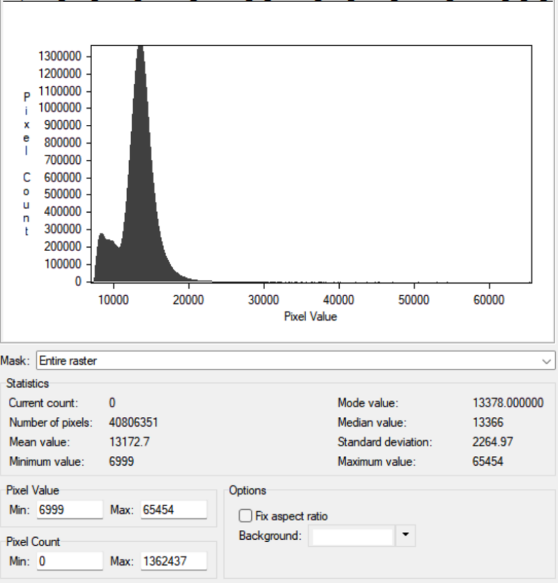
To describe the Landsat 9 Shortwave Infrared 2 band (Band 7), we examine the provided image statistics and the histogram distribution. This band is composed of 40,806,351 pixels with a mean value of 13,172.7 and a median of 13,366. The histogram shows a very sharp peak centred at a mode of 13,378, with a small "shoulder" of lower values to the left. While the data technically reaches a maximum of 65,454, the vast majority of the pixels are clustered in a very narrow range around 13,000. This tells us that the raw data lacks contrast; because most pixels have nearly identical brightness levels, the image likely appears dark and dull, making it hard to see specific features on the ground. To improve the visual quality of this band, a linear contrast stretch is a necessary enhancement. This technique takes the narrow group of values where the majority of the data is located and spreads them out across the full display range (0–255). I reason that Band 7 is specifically useful for identifying things like mineral deposits or charred earth after a fire, but these details are "buried" when the data is so tightly packed. By stretching the contrast, we can separate these subtle shades of gray, allowing the human eye to actually see the patterns and boundaries that the sensor has captured.
Create Your Own Website With Webador